Ordinary Least Square (OLS) in EViews and its Interpretation

In the Regression analysis of Econometric first of all, we should have to calculate OLS.
Because OLS is most essential for the following reasons.

• it is one of the simplest methods to measure Regression.

• widely used to estimate the parameter of a linear regression model.

• it minimizes the sum of the squared errors.so we can say that is one that has minimum variance.

• it is used to model the relationship between a continuous response variable y and an explanatory variable x.

• it is an unbiased Estimator.

• it is concerned with the squares of the errors.

OLS is called that it has a property of BLUE (Best, Linear, Unbiased, Estimator).

Now we are moving towards the solution and finding of OLS by E-views.

1. Import the data from the Excel sheet and then by clicking the right-hand button from the mouse you can see the "paste" command just click on it.

      2. Select the Dependent (DV) and independent variables(IVs).

       3. By Putting Cursor on Selected Variables, Right-click from muse then selects "open" then "Group" after that click on it. Now your new window will be like that,

       4. Now click in "Quick" from the Manue Bar.

      5.  Now Select "Estimate Equation" from these options. then the new window will be open and would be like as follows.

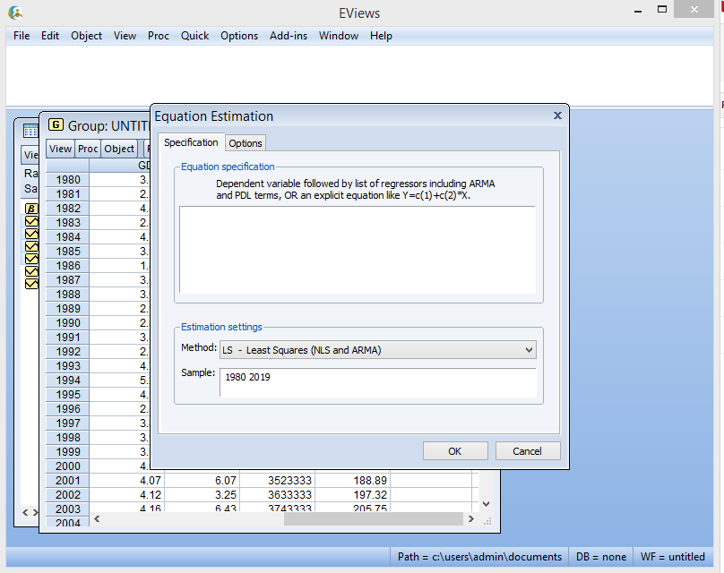
      6. Put your DV and IVs here with constant (c) in the equational form. the demo will be as follows. After putting variables click on OK.

    7. After click results of OLS will be displayed on your screen. Like as

--------------------------------------------------------------------------------------------------------------------------

Now we are going to Interpret the Result completely.

Dependent Variable: GDP Method: Least Squares Date: 02/13/20   Time: 22:48 Sample: 1980 2019 Included observations: 40
Variable	Coefficient	Std. Error	t-Statistic	Prob.
C	3.633130	1.449609	2.506284	0.0169
INFLATION	-0.199112	0.085762	-2.321683	0.0260
PRICES	0.010102	0.017605	0.573820	0.5697
POPULATION	-9.83E-08	1.37E-06	-0.071797	0.9432
R-squared	0.491027	Mean dependent var		4.005952
Adjusted R-squared	0.448612	S.D. dependent var		0.829710
S.E. of regression	0.616105	Akaike info criterion		1.963840
Sum squared resid	13.66507	Schwarz criterion		2.132728
Log likelihood	-35.27681	Hannan-Quinn criter.		2.024905
F-statistic	11.57688	Durbin-Watson stat		2.041251
Prob(F-statistic)	0.000018

Above mentioned randomly values are taken from the web. We have 40 observations. from the year 1980 to 2019. We have the following results,

Ho: there is no association between GDP and Inflation, Prices and Population.

Ha: there is some no association between GDP and Inflation, Prices and Population.

Results.

When P-value is less than 5% then we accept the alternative hypothesis. Now we can observe that GDP has negative signification relationship with inflation and negative in-significant relationship with the population. Meanwhile have positive in-signification relation with the price.  R-Square clarifies that our independent variables are explaining 49% variation of our dependent variable. Our F-static is higher than our Prob (F-static) which explains that our independent variables (price, inflation, and population) are jointly affecting our dependent variable (GDP). Hannan criter and Durbin Watson stat is more than 2 which indicates us there is no problem of auto-correlation prevailing in our model.  Average (mean) of the dependent variable is 4.00s whereas mean can be deviated from its central point by 0.82.  The standard error of regression explains the deference of the actual and estimated value of the dependent and independent variables. So here S.E of regression explains the difference between actual and estimated value has 0.61 differences.